Geometry objects: representation, parametrization and mapping#
A vector of values (unknown parameters or data) in the Bayesian Inverse problem setting can be interpreted in various ways. It can be, for example, a vector of function values at 1D or 2D grid points, a vector of image pixels, a vector of expansion coefficients, or a collection of variables, e.g. the temperature measurement at four cities: A, B, C, and D.
In CUQIpy, the cuqi.geometry module provides classes for different representations of vectors, e.g Continuous1D, Continuous2D, Image2D, and Discrete.
Here we explore geometry assignment for Distributions, Samples and CUQIarray. We explore the three main functionalities of the geometry objects: representation, parametrization, and mapping.
Variable representation #
First let us create 1000 samples from a 4-element distribution \(y\):
Show code cell content
from cuqi.distribution import Gaussian
from cuqi.geometry import Image2D, Discrete, StepExpansion, MappedGeometry
from cuqi.array import CUQIarray
import numpy as np
mu = np.array([5, 3, 1, 0])
sigma = np.array([1, 2, 3, 0.5])
y = Gaussian(mean=mu, cov=sigma**2)
y_samples = y.sample(1000)
If no geometry is provided by the user, when creating a Distribution for example, CUQIpy will assign _DefaultGeometry1D (trivial geometry) to the distribution and the Samples produced from it.
print(y.geometry)
print(y_samples.geometry)
_DefaultGeometry1D(4,)
_DefaultGeometry1D(4,)
Samples are plotted with line plot by default, which is due to how the _DefaultGeometry1D interprets the samples.
y_samples.plot([100,200,300])
[<matplotlib.lines.Line2D at 0x7fd901344dc0>,
 <matplotlib.lines.Line2D at 0x7fd901344eb0>,
 <matplotlib.lines.Line2D at 0x7fd901344fa0>]
We may equip the distribution with a different geometry, either when creating it, or afterwards. Let us for example assign an Image2D geometry to the distribution y. First we create the Image2D geometry and we assume the shape of the image is \(2\times2\):
geom_image = Image2D((2,2))
print(geom_image)
Image2D(4,)
We can check the number of parameters (parameter dimension) of the geometry:
geom_image.par_dim
4
We can also check the shape of its representation (size of the image in this case) using the property fun_shape:
geom_image.fun_shape
(2, 2)
Now we equip the distribution y with this Image2D geometry.
y.geometry = geom_image
Check the geometry of y:
y.geometry
Image2D(4,)
With this distribution set up, we are ready to generate some samples
# call method to sample
y_samples = y.sample(50)
We can check that we have produced 50 samples, each of size 4:
y_samples.shape
(4, 50)
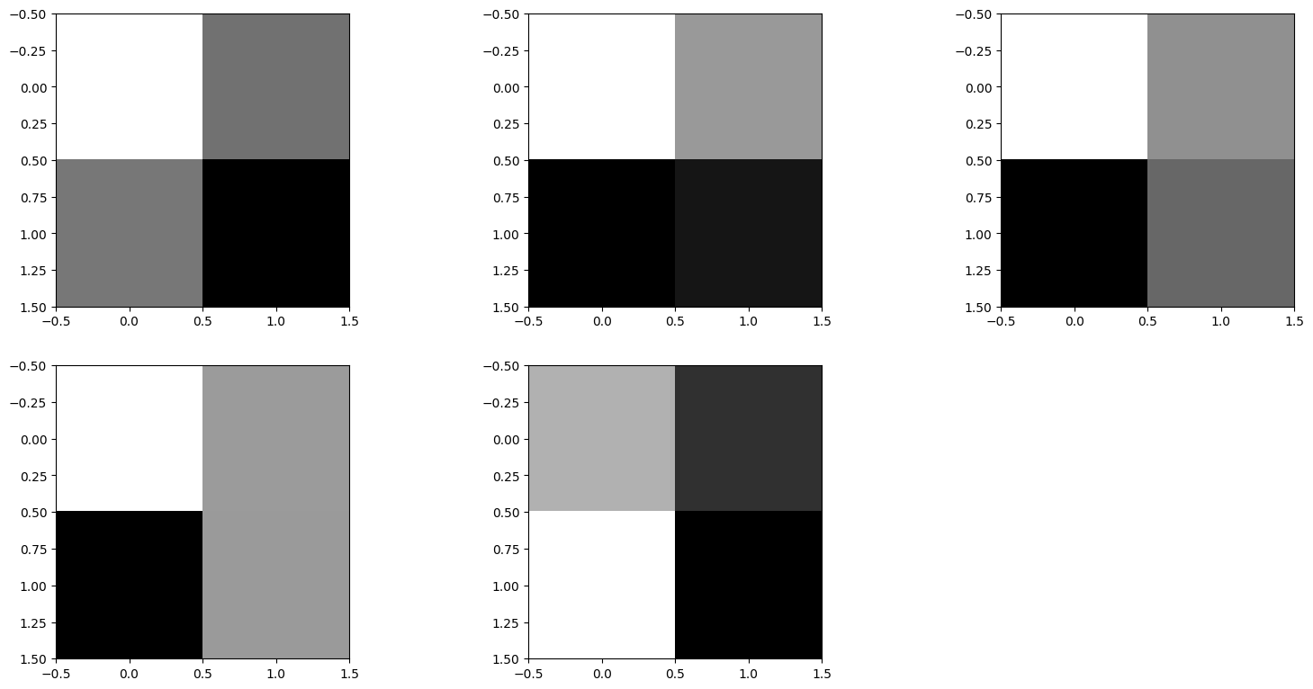
We plot a couple of samples:
y_samples.plot()
Plotting 5 randomly selected samples
[<matplotlib.image.AxesImage at 0x7fd9013949a0>,
 <matplotlib.image.AxesImage at 0x7fd8ff245f60>,
 <matplotlib.image.AxesImage at 0x7fd8ff27af80>,
 <matplotlib.image.AxesImage at 0x7fd8ff2b6cb0>,
 <matplotlib.image.AxesImage at 0x7fd8ff116cb0>]
What if the 4 parameters in samples have a different meaning? For example, the four parameters might represent labelled quantities such as temperature measurement at four cities A, B, C, D. In this case, we can use a Discrete geometry:
geom_discrete = Discrete(['Temperature A', 'Temperature B', 'Temperature C', 'Temperature D'])
print(geom_discrete)
Discrete(4,)
We can update the distribution’s geometry and generate some new samples:
y.geometry = geom_discrete
y_samples = y.sample(100)
The samples will now know about their new Discrete geometry and the plotting style will be changed:
y_samples.plot();
Plotting 5 randomly selected samples
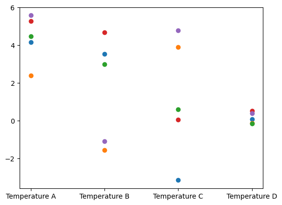
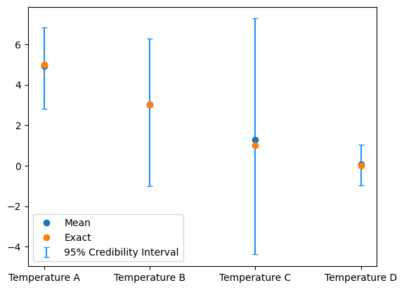
The credibility interval plot style is also updated to show errorbars for the Discrete geometry:
y_samples.plot_ci(95, exact=mu)
[<matplotlib.lines.Line2D at 0x7fd8fe5c3880>,
 <matplotlib.lines.Line2D at 0x7fd8fe5c3010>,
 <ErrorbarContainer object of 3 artists>]
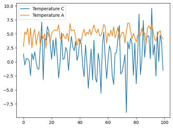
And similarly, in the chain plot, the legend reflects the particular labels:
y_samples.plot_chain([2,0])
[<matplotlib.lines.Line2D at 0x7fd8fe677040>,
 <matplotlib.lines.Line2D at 0x7fd8fe677130>]
Varible parameterization #
In CUQIpy we have geometries that represents a particular parameterization of the variables (e.g. StepExpansion, KLExpansion, etc).
For example, in the StepExpansion geometry, the parameters represent expansion coefficients for equidistance-step basis functions. You can read more about StepExpansion by typing help(cuqi.geometry.StepExpansion) in a the code cell below or by looking at the documentation of StepExpansion
Let us create a StepExpansion geometry, we first need to create a grid on which the step functions are defined, let us assume the grid is defined on the interval \([0,1]\):
grid = np.linspace(0, 1, 100)
Then we create the StepExpansion geometry with 4 steps and assign it to the distribution y:
geom_step_expantion = StepExpansion(grid, n_steps=4)
y.geometry = geom_step_expantion
print(y.geometry)
StepExpansion(4,)
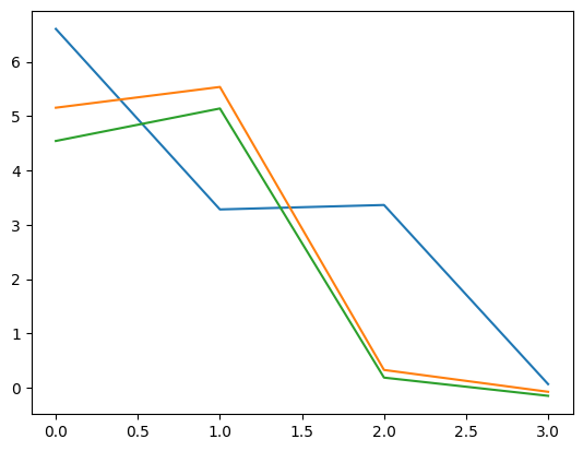
Let us samples the distribution y and plot the samples:
y_step_samples = y.sample(100)
y_step_samples.plot()
Plotting 5 randomly selected samples
[<matplotlib.lines.Line2D at 0x7fd8ff08ba00>,
 <matplotlib.lines.Line2D at 0x7fd8ff08baf0>,
 <matplotlib.lines.Line2D at 0x7fd8ff08a950>,
 <matplotlib.lines.Line2D at 0x7fd8ff08bbb0>,
 <matplotlib.lines.Line2D at 0x7fd8ff08bca0>]
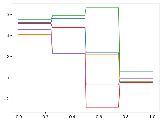
Note that the samples are now represented as expansion coefficients of the step functions.
Examples of using StepExpansion and KLExpansion geometries in the context of a PDE parameterization for a heat 1D BIP can be found here, and here [ARA+24], respectively.
Variable mapping #
In CUQIpy, we provide the MappedGeometry object which equips geometries with a mapping function that are applied to the variables, this mapping can also be viewed as parametrization. An example of a commonly used mapping in inverse problems is \(e^x\) for unknown parameters \(x\) to ensure positivity regardless of the value of \(x\).
Let us use the MappedGeometry to map the StepExpansion geometry we created earlier with the exponential function:
geom_step_expantion_mapped = MappedGeometry(geom_step_expantion, map=lambda x: np.exp(x))
Let us again, assign the MappedGeometry to the distribution y and generate samples and plot them:
y.geometry = geom_step_expantion_mapped
y_mapped_step_samples = y.sample(100)
y_mapped_step_samples.plot()
Plotting 5 randomly selected samples
[<matplotlib.lines.Line2D at 0x7fd8fef21000>,
 <matplotlib.lines.Line2D at 0x7fd8fef210f0>,
 <matplotlib.lines.Line2D at 0x7fd8fef211e0>,
 <matplotlib.lines.Line2D at 0x7fd8fef212d0>,
 <matplotlib.lines.Line2D at 0x7fd8fef213c0>]
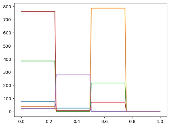
Note that the samples are still representing the expansion coefficients of the step functions, but the mapping function \(e^x\) has been applied to the samples. All samples are now non-negative.
★ Elaboration: Specifying a Geometry object for CUQIarray objects:#
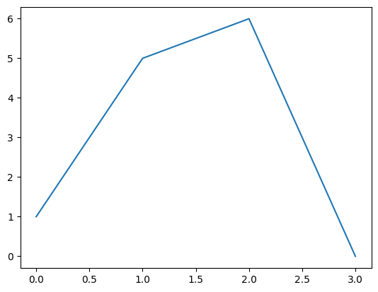
Geometries can also be specified for CUQIarray, the basic array structure in CUQIpy. Let us create a CUQIarray object with four parameters as follows:
q = CUQIarray([1,5,6,0])
We look at the geometry property
q.geometry
_DefaultGeometry1D(4,)
And then let us plot our variable q:
q.plot()
[<matplotlib.lines.Line2D at 0x7fd8fefbd360>]
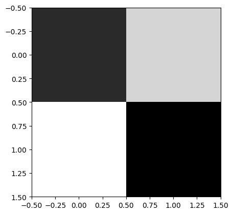
We now choose a different interpretation for the variable q by changing its geometry to, for example, the Image2D geometry we created, and then we plot:
q.geometry = geom_image
q.plot()
[<matplotlib.image.AxesImage at 0x7fd8feffa980>]
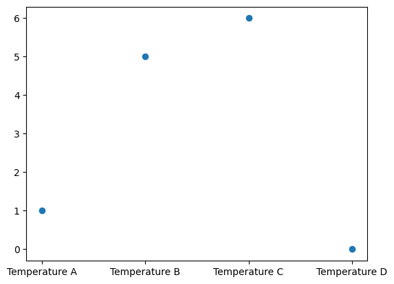
Finally we set the Discrete geometry we created as the geometry for q and plot:
q.geometry = geom_discrete
q.plot()
[<matplotlib.lines.Line2D at 0x7fd8feec5480>]